History of Money: from Barter to Banknotes
Money by itself is nothing but a piece of paper or a coin. The value of money is the value assigned to it, and has nothing to do with the actual value of the paper. It is a medium of exchange, used in trade of goods or services or for purchases. It is exchanged for a certain measured or determined value equivalent to the substance or underlying the one exchanged.
Money is accepted worldwide as a form of payment or payment for exchange of goods or services. Let us understand how it evolved and how it is used today.
Money was being used for more than 3000 years in some or other forms and before that time, system of bartering was being used. In barter system, goods were used to be exchanged for other goods. Goods were used as a consideration in order to complete the transaction. For example livestock, sheep or sack of grain were used for exchange against the other commodities. Services involving labours were compensated for exchange of food provided to them.

It is believed that the Chinese were the first to use the barter system, 3000 years ago. They traded weapons and tools as a medium of exchange which they eventually abandoned as it was difficult to carry around. They subsequently converted into tiny small round coins of the metals. Some scholars believe that Chinese currency dates back 4500 years ago (which was termed as the New Stone Age) when trading of goods was based on cowry shells as a currency. The countries in other continents such as Australia, Africa, and America have also used cowry shells as currency in past. However, the first minted coins were used in Lydia which is now in western Turkey. Few hundred years later, Lydia’s King Alyattes minted the first official currency. The coins were made from electrum, a mixture of silver and gold that occurs naturally, and stamped with pictures that acted as denominations. Based on the size, picture or nature, the specific value was assigned to the coin. The Lydians minted the coin for the first time in 600 BC. The coins are still popular and in use since the metal is still available, and based on the cost of the metal, the value can be easily assigned to the coin.
The shift to paper money in Europe increased the amount of international trade that could occur. Banks and the ruling classes started buying currencies from other nations and created the first currency market. The stability of a particular monarchy or a government affected the value of the currency of a country and the ability of that country to trade in an increasingly international market.
Exchange Rate

Figure 2.1 Balance between Currencies
The exchange rate is different based on the date on which the transaction is carried. The spot exchange rate refers to the current exchange rate. The forward exchange rate refers to an exchange rate that is quoted and traded today, but the date of transaction, the delivery and payment, is sometime on a future date.
In the retail currency exchange market, a different buying rate and selling rate are quoted by the money dealers. The buying rate is the rate at which the money dealers will buy foreign currency and the selling rate is the rate at which they will sell the currency.
Determinants of Exchange Rate
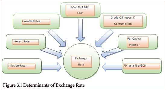
Numerous factors determine exchange rates. These rates are related to the trading relationships between the two countries. Exchange rate is relative and is expressed as a comparison of the currencies of two nations. The exchange rate also conveys the relative strengths of the economies of the two countries. Some of the major principle determinants of exchange rates between the two countries which influence the exchange rate areas follows:
1. Interest Rate
2. Inflation Rate
3. Growth Rates
4. CAD as a % of GDP
5. Crude Oil Import and Consumption
6. Per Capita Income
7. FDI as a % of GDP
8. Political Stability, Economic Performance and Act of God
ASSUMPTIONS OF INR/USD ANALYSIS

Figure 3.1 Determinants of Exchange Rate
Each determinant has a direct or an inverse impact and a definite relationship with the exchange rate. In our analysis, we have considered top 7 determinants which can be quantified. Following are a few assumptions of the INR/USD analysis:
1. Political stability and economic performance cannot be quantified completely. Therefore, we have considered only the quantifiable portion [For example, the Foreign Direct Investment (FDI) policy of both the countries] as the FDI figures are available for both the countries. We have not considered the non-quantifiable portion relating to political stability and economic performance.
2. Both periods i.e., the pre-LPG and post-LPG period have been taken into account. In the pre-LPG period, we have considered the period between 1980 to 1991 (when India had a relatively closed economy) and in the post-LPG period we have considered period between 1991 to 2016 (when India had opened up for liberalization, privatization and globalization).
In the short term analysis, we have covered the period of 2000 to 2016.
3. We have built a mathematical model based on the impact of all quantifiable variables on the exchange rate.
Calculation of Long Term and Short Term Rate by Mathematical Model
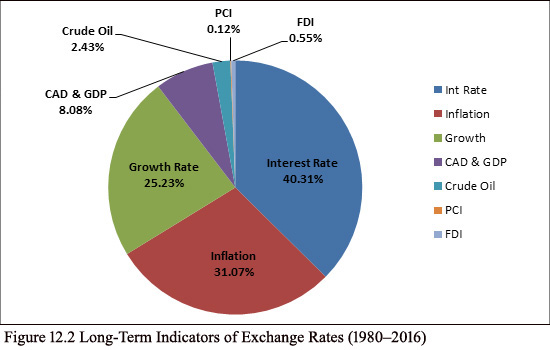
In the mathematical model, we have tried to explain the movement of exchange rate with the help of the seven factors which have been discussed earlier. We have populated the data for both the countries, i.e., India and the USA and we have worked out the difference of each factor between both the countries.
We have plotted differentials of the following seven factors in Table 12.1.
1. Interest rate
2. Inflation
3. Growth
4. CAD as a % of GDP
5. Crude oil consumption in relative terms
6. PCI in negative terms
7. FDI as a % of GDP
We have assigned positive or negative signs according to their direct or inverse correlation with the exchange rate. Positive sign in a difference column of all the seven factors will indicate that rupee will appreciate against the dollar and the negative sign in the difference column of all the seven factors will indicate that rupee will depreciate against the dollar.
We have added all these difference values of all seven factors and have arrived at the net differential rate for every year. This differential rate implies the movement of exchange rate during the year, i.e., from previous year to the current year. The multiplier is derived from the differential rates of the above seven factors which is explained later. The previous year’s exchange rate has been multiplied with the multiplier which was arrived at every year to get the exchange rate of the current year. Similarly, we have plotted exchange rate as per the mathematical model of the table and we have compared it with actual exchange rate.


Calculation of Short Term Exchange Rate by Regression -
Regression is a statistical measure that attempts to determine the strength of the relationship between one dependent variable and a series of other changing variables.Carrying out this exercise for a long term would not be appropriate since the long term would include years when India was a relatively closed economy and was strictly regulated by the Reserve Bank of India and the government. It was only in 1991 that the Rupee was devalued and the economy became open with Liberalization, Privatization, and Globalization (LPG). This would lead to a drastic change in the indicators of the exchange rate. Thus, long-term regression will not give the true picture of the degree of dependency of these changing variables (due to strict regulation and control) with the exchange rate. Therefore, the same has not been calculated.
Regression module can be downloaded in the MS Excel and one can define the y-axis (variable to be predicted) and the x-axis (all dependent variables).
Once we select this we will get full results automatically and all predicted values of the results in a different table.
Explanation of Terms:
These are the ‘Goodness of Fit’ measures. They tell us how well the calculated linear equation fits our data. They are discussed as follows:1. Multiple R: This is the correlation coefficient. It tells us how strong the linear relationship is. For example, a value of 1 means a perfect positive relationship and a value of zero means no relationship at all. It is the square root of R square.
2. R square: This is R2, the coefficient of determination. It tells you how many points fall on the regression line. The closer it is to 1, the better the regression line fits the data.
3. Adjusted R Square: The adjusted R-squared adjust for the number of terms in a model. You’ll want to use this instead of R square if you have more than one x variable.
4. Standard Error: An estimate of the standard deviation of the error μ. This is not the same as the standard error in descriptive statistics. The standard error of the regression is the precision in which the regression coefficient is measured—if the coefficient is large compared to the standard error, then the coefficient is probably different from 0.
5. Observations: Number of observations in the sample.
6. ANOVA: Analysis of variations
7. df= Degrees of freedom
8. ss = Sum of squares.
9. Regression ms= Regression ss/regression degrees of freedom.
10. Residual ms= Mean square error (Residual ss/residual degrees of freedom).
11. F: Overall F test for the null hypothesis.
12. Significance F: The associated P-Value to check if your results are reliable (statistically significant). If this value is less than 0.05, we are fine.
REGRESSION COEFFICIENTS
This section, 'Regression Coefficients' of the table gives us very specific information about the components we choose to put into our data analysis. Let us discuss in detail.
1. Coefficient: Gives us the least squares estimate.
2. Standard Error: It is the least squares estimate of the standard error.
3. T Stat: The T Statistics for the null hypothesis vs. the alternate hypothesis.
4. P Value: It gives us the P-value for the hypothesis test. Most or all P-values should be below 0.05.
5. Lower 95%: The lower boundary for the confidence interval.
6. Upper 95%: The upper boundary for the confidence interval.
Need for Forecasting Exchange Rate

Techniques for Managing Currency Exposures and Risks -
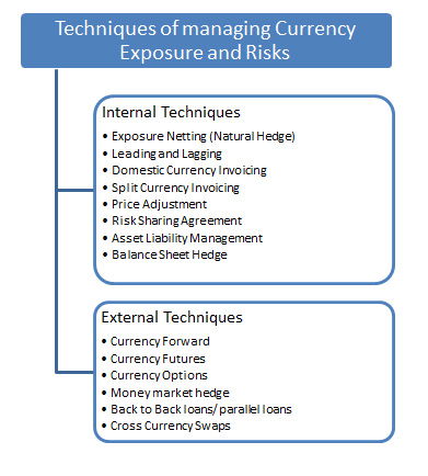
Currency exposure can be managed by using Internal or external techniques or a combination of both. The former include all those techniques where business enterprise undertake some operational changes and such changes do not require assistance of banks or financial institutions. On the other hand external techniques of managing currency exposure necessarily involves assistance of an external party in the form of banks or financial institutions. Netting the exposure, leading or lagging the payment or receipts, changing the currency of invoicing are some of the examples of internal techniques where as buying or selling of derivative products such as futures, forwards, options with the assistance of a bank or financial institution are some of the examples of external techniques. When choosing between different types of hedging the business enterprise must compare costs, taxes, effects on accounting conventions (important for translation) and regulation (which may limit some transactions). Before using the external techniques, business enterprises should consider which internal hedging method is open to it and at what cost.